What is a climate model? What are the models’ first conclusions?

Climate models

The future climate of the Earth will probably evolve in a way totally unprecedented since our species has begun its terrestrial existence. As it is thus impossible to infer from the sole observation of the past what can happen “later”, the only tools that the scientific community has in hands to try to know what will happen in the future are climate models.

A climate model is nothing more (some scientists might find that it’s not that bad already !) than a complex software which aims to reproduce as faithfully as possible the real climate system. It is therefore a large computer program, built the following way:

• competent scientists select, within the climate system or one of its major components, and everyone for the part (s)he works on, a couple of parameters that are considered as sufficient to characterize in a satisfactory way the system – or the sub-system – for the question studied (which is the long term evolution of the climate system). These parameters will typically include the annual mean temperature and the corresponding spatial pattern, the mean precipitations and the corresponding spatial pattern, the local vegetation and its carbon content for each major region, etc,

• the rules that drive the evolution of a given parameter according to the others variables are then formalized, for example the rate of evaporation is expressed as a function of the temperature, the wind speed, the vegetation taking place on the ground (or the water temperature for the ocean), etc. Rules that must always be satisfied are also included (such as energy conservation),

• then a stage of computer programing takes place, which means that the rules stated above are turned into lines of computer code,

• as it is not possible to describe what is happening absolutely everywhere with a computer (it would require an infinite number of points, and computers don’t like infinite numbers very much), models work with a grid: the planet is covered with an imaginary net, with the size of the mesh (like for fishing nets, the mesh is the distance that separates two threads) being typically a couple of hundred kilometers (depends on the model and the time of design),

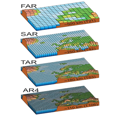
Evolution of the resolution (or of the size of the mesh, it’s all the same) of global climate models with time.

Before the IPCC First Assessment Report (noted FAR), that is in the 1980’s, the mesh was typically 500 km wide. Some regional models allowed meshes of 50 km or so in a particular region but then the meshes would strech to up to 1000 km for the rest of the world.

At the time of the IPCC Second Assessment Report (SAR), in 1995, the size of the mesh had been divided by two, and today, at the time of the AR4 (that stands for 4th Assessment Report, released in 2007), it underwent an additional division by two compared to 1995.

Source : IPCC, 4th assessment report, 2007

• As our world is in three dimensions, actually it is not divided in little squares but rather in little “shoe boxes”, with several tenths of “boxes” along the vertical,

• The computer is explained what is inside each “box” (air, water, ground, vegetation, clouds, etc, graph below),

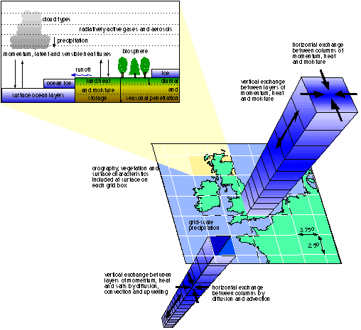
Global view of a climate model, also called “global circulation model” or GCM.

Source: Hadley Centre.

• for each node of the three dimensionnal netting, or the interior of each box (that depends on the parameter), the initial situation is described, by indicating the value of the parameters that the computer will work with: temperature, pressure, humidity, cloud cover, wind, salinity for the sea water, etc.

• then the model does a “run”, that is the computer calculates, on the grounds of the equations included in the model and the initial values, how the situation evovles at the nodes of the netting at regular time intervals (depending on the available processing power, the time intervals will be half hours or months !).

One of the advantages of computer models is that they can easily include an additional perturbation that evolves with time, for example the increase of greenhouse gas concentration in the atmosphere, to perform a virtual comparison of what happens “if”. “all there is to do” is to add an equation in the list.

Modelling is a discipline that did not start yesterday: it took its rise in the 60’s (the first atmospheric model was implemented on the first computer, the ENIAC). What enabled a soaring of the discipline is more the tremendous increase of the available processing power (and the availability of stallite data to confront model runs to observations) than breakthroughs in physics, what was pretty well known already a couple of decades ago.

For example, the time required to simulate one month of future climate has been divided by 100 between 1980 and today !

The more powerful the computers are, and the smaller the meshes can be. The shorter the prediction horizon is, and the smaller the meshes can also be, what increases the reliability of the predictions: meteorologists, that are not interested in the weather to be in a couple of centuries, but in the weather for tomorrow or after-tomorrow, work with models that are rather similar to those used by climatologists, but with meshes only a couple km wide.

How many models ?

There are now about 15 different global circulation models around the world, designed and operated by as many teams of scientists (a major country has 2 to 3 teams/models), the whole representing about 2.000 individuals. But the total number of scientists, coming from various disciplines, that contribute to the construction or the feeding of a model is ten times superior at least: in order to know “what to put in the box”, it is necessary to use previously published work from many physicists, chemists, biologists, geologists, oceanographists, aerologists, glaciologists, demographs…

The laws of physics remain obviously the same everywhere and all the time, but these models are still rather different one from another, especially for the processes that are not explicitely taken into account, but are managed with parameters: some represent clouds this way, others that way, some take into account the biosphere feedbacks this way, others do not at all or represent them that way, etc

In France, a large deal of climate simulations are performed within the Institut Pierre Simon Laplace (IPSL), that rassembles:

• The Laboratoire de Météorologie Dynamique du CNRS
• The Laboratoire des Sciences du Climat et de l’Environnement
• The Laboratoire d’Océanographie Dynamique et de Climatologie
• The Laboratoire Atmosphères, Milieux, Observations Spatiales
• The Laboratoire de Physique et Chimie Marines (no web site, as amazing as it may seem !)

What do models take into account ?

All the models do not take exactely the same things into account, though they all have a common basis. Some will represent clouds in such a way, others in another, some will parametrize a given process (which means that it does not respond dynamically to what happens elsewhere in the model), others will not, etc. The major difference between models, however, comes from their year of conception.

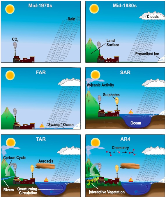
Evolution of the degree of sophistication of the global models since the 1970’s.

At first, models where purely atmospheric, representing the evolution of air temperatures and precipitations under the forcing of additional CO2 into the air. In the 1980’s came land occupation, clouds (parametrized), and sea iced (prescribed means not coupled to the rest). At the time of the IPCC First Assessment Report (FAR), ocean was there, but without any large scale circulation taken into account.

At the time of the Second Assessment Report (SAR, 1995) models “welcomed” aerosols, volcanic activity and large scale horizontal circulation of the ocean. At the time of the Third Assessment Report (TAR), in 2001, those tools also took into account the ocean overturning, something of the carbon cycle, and rivers.

At last, some models used to write the 4th Assessment Report (AR4, 2007) include some atmospheric chemistry (that is processes that allow to represent the atmospheric increase – or decrease – of a coumpound A from the variation of the abundance of coumpounds B and/or C), and a dynamic vegetation, reacting in accordance to regional climate conditions.

What is remarkable is the fact that this major complexification of the tools used has not changed the major conclusions given in the 70’s: if our emissions lead to doubling of the CO2 in a century, it will modify the climate system, and in particular lead to a mean temperature increase of a couple °C.

Source : IPCC, 4th Assessment report, 2007

If we take a deeper look, here are the principal processes that are represented in the models (between parenthesis it is specified whether some models only or all models take the corresponding process into account). Caution ! “Represented” does not mean that everything is known on the process, and that the way it is represented in the model is perfect, but just that it is taken into account, in a way or another, in the model:

• energy exchanges between the ground, the ocean, the atmosphere, and space, be it through electromagnetic radiation, sensible heat, or latent heat (all models).

• the radiative transfers in the atmosphere, that is the way solar and terrestrial radiance pass through the atmosphere or are absorbed by the various greenhouse gases it contains,

• the large-scale atmospheric circulation, and therefore the associated water transportation (all models),

• the large-scale oceanic circulation, both horizontal and overturning (all models), and the interactions (energy exchanges, water exchanges) between ocean and atmosphere (all models),

• the buildup and melting of sea ice (all models),

• clouds (all models), but a correct representation of clouds remains one of the “hard points” of modelling,

• the elementary carbon cycle, that is carbon exchanges between the ocean, the terrestrial ecosystems, and the atmosphere (all models, but with a wide range of complexity), and, for the most advanced, feedbacks of a climate change on the vegetation.

What are their weaknesses ?

The three main sources of incertitude in the climate models are the following:

• First of all the atmospheric part of the system is not entirely foreseeable. It’s the reason why weather forecasts, obtained with something which is very much alike the atmospheric part of global models, sometimes prove wrong, even if statistically they are generally right (even if our attention is mainly focused on the mistakes, as always !),

• Then there are non avoidable simplifications when a model is designed. It is nevertheless legitimate and frequent to do so: the simple fact that a simplification exists is not necessarily a source of error. For example, the blueprint of a building to be constructed does not reproduce all the details of the future building, but only the “most important things”: does that prevent to have a good idea of the facility with which one will move inside the building ?

• they still represent only partially the climate system (but scientists consider that it does not question the main qualitative conclusions). Among the elements that need to be better taken into account, one can mention:
  • clouds (because they are objects of small size relatively to the size of the mesh, therefore it is not possible to manage them explicitely but they are treated with approximations),
  • sources and sinks of oceanic and continental carbon, and notably the influence of the biosphere (that is all living beings) on the carbon cycle,
  • continental evaporation, which also involves many small scale processes,
  • deep oceanic circulation (that is difficult to measure, which means that it is difficult to compare what the model says with observations),
  • the methane cycle (methane is the gas linked to putrefaction), and that of nitrous oxide,
  • the consequences of the increase of tropospheric ozone (the one close to the ground),
  • the role of organic or mineral aerosols (dust, soot…),

But one should not deduct from the fact that some “haze” remain that all the results of simulations can be just throwed away ! Actually the comparisons available in the scientific litterature tend to confirm more and more that models are trustworthy.

First conclusions of simulations

An essentiel point is that, even if they are all slightly different one from another in their conception, and even if the quantitative results they yield are not rigorously identical, all the models come to the same conclusion: humankind modifies the climate system and globally increases the average near ground temperature. In addition these models also indicate that the humane influence will increase if the present trends go on for greenhouse gases emissions.

• The average near ground temperature will increase (figure below). Depending on the emission scenario chosen, we speak of something between 1 and 6 °C in a century’s time.

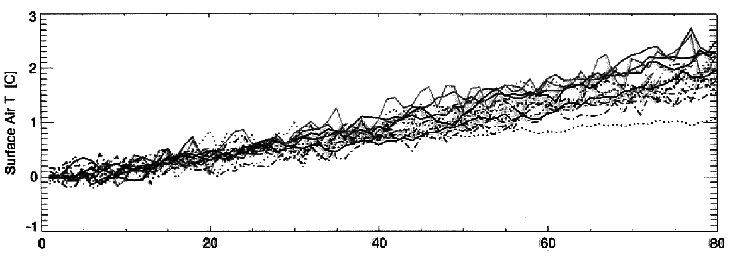
This figure represents the evolution of the average near ground temperature (which is often called the “average temperature of the earth”) for most of the world’s models (one curve per model) that have all been given the same hypothesis of a CO2 concentration increasing of 1% per year (which is roughly the present rate of increase).

The zero of the horizontal axis – graduated in years – corresponds to the start of the run of the models, and the 0 of the vertical axis, graduated in degrees, corresponds to the difference between the average temperature for each year with the value at the start of the run.

Sources : PCMDI/IPSL

• Water exchanges between the ground (and the ocean) and the atmosphere will globally increase (graph below). This can be simply explained by the fact that when the air is globally hotter, it is able to contain more water vapour, and therefore evaporation is more important in a hotter climate. Well, as water does not accumulate in the atmosphere, what goes up must come down, and more evaporation results in more rain (and inversely during ice ages, when the global climate is much cooler, it is also much dryer). This means than it will globally rain more often, or…more intensely (with an increase of the risk of floods in the latter case).

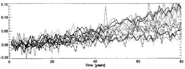
The above figure represents the evolution of the annual precipitations for the whole world (one curve per model, as for the previous box) that have all been given the same hypothesis of a CO2 concentration increasing of 1% per year.

The zero of the horizontal axis – graduated in years – corresponds to the start of the run of the models, and the 0 of the vertical axis, graduated in millimeters of water per day, corresponds to the difference between the average temperature for each year with the value at the start of the run.

When a curve goes over the 0,05 value on the vertical axis, for example, it means that the precipitations on earth have increased, on average, of 0,05 mm per day, that is 18 mm per year, or 3,5% of the present average precipitations (520 mm of rain per year, on average for the whole planet).

But this surplus of rain will not be evenly dispatched: most models predict a great variability depending on the latitude (below).

Sources: PCMDI/IPSL

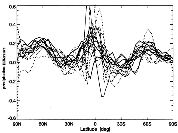
The above figure shows the “response” of the models (one curve per model, just as above) to a doubling of the atmospheric CO2 (in 60 to 80 years if we prolongate the trends) regarding the precipitations depending on the latitude. The vertical axis represents the difference between the average daily precipitation in the future and the present one (daily average for the whole planet), in mm of water.

It can be seen that, for example, around 60° North (Northern Scotland, Southern Norway, where rain is not scarce), it would rain even more (an additionnal 70 mm of rain per year), while around 30°N (California, Sahara, Mongolia, that is places not overwhelmed by rain today) it would rain the same or a little less, and around 30 °S (South Africa, Australia, Argentina) it would rain a little less.

Sources: PCMDI/IPSL

• And at last the temperatures will globally rise more:
  • during the night (opposed to the day),
  • during the winter in the middle latitudes (opposed to summer),
  • near the poles (opposed to the mid-latitudes and the intertropical region),

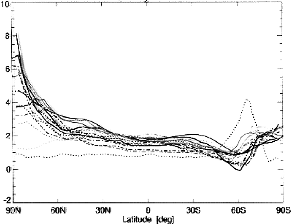
The above figure shows the average temperature rise depending on the latitude (one curve par model, just as above) when the atmospheric concentration of CO2 has doubled (in 60 to 80 years if we prolongate the trends)

We can see that sea ice close to the northern pole (90° N, on the extreme left) will be put under pressure: the temperature rise could reach 8° C in that region.

Sources: PCMDI/IPSL

The characteristics mentionned above have the same origin: the greenhouse effect, which consists in trapping part of the infrared radiation of the Earth, does not vanish or greatly decrease at night or during the winter, as the heating of the sun does. Consequently, when the sun is not heating the surface (or is heating it much less, as in winter), the indirect heating of the ground coming from the greenhouse effect becomes an important or dominant term. Therefore the relative effect of the enhancement of this greenhouse effect is higher when there is no sun (winter and night). Another process comes into effect: when there is no sun, the air is cooler or colder, thus dryer, and the “natural” greenhouse effect coming from water vapour is lower. Therefore the consequence of an additionnal greenhouse effect coming from an increase of the CO2 concentration (which is well mixed and not dependant on temperature) is proportionnaly higher where/when the temperature is low. Both these processes explain part of the higher increase near the poles.

• Over the continents (as opposed to over the oceans), because the thermal inertia of large water masses is much greater than that of the ground ; the increase over the Northern Hemisphere continents might be 1,5 to 2 times as fast as the global increase. It means that if the average near ground air temperature increases by 3 °C in 2100, which remains compatible with the known fossil fuel resources, a 5° C increase might occur over large continental zones. And if “everything goes wrong”, the average near ground air temperature could increase by 8 to 9 °C within a couple centuries…

Want to know more ? Additional information can be found on this other page.